Introduction to Neural Inverse Design of Nanostructures (NIDN)
Welcome to the notebook describing Neural Inverse Design of Nanostructures (NIDN).
NIDN is a Python package for inverse design of nanostructures using neural networks, powered by PyTorch. With NIDN, the user can find configurations of three-dimensional (nano-)structures and metamaterials that match certain desirable properties, for instance the reflection and absorption of light at certain wavelengths.
For this notebook, we will showcase one example of how NIDN can be used. Together with our Torch-based Rigorous Coupled-Wave Analysis (TRCWA) simulation tool, which is based on the GRCWA package made by Weiliang Jin, we can find a structure that meets our requirements for reflection, transmission, and absorption, e.g., as for the example shown below.
# Picture of an example plot here
### NB: The legend should not say *Produced* Reflectance!
#
Important information and core settings in NIDN
You might notice the word cfg a lot in the TRCWA code. The config
class cfg contains all of the parameters the user would need while
using TRCWA and makes setting up the inverse design process much more
convinient. Feel free to check it out in our
documentation. TODO: Link
to doc page where all config parameters are explained.
Below are some core details and settings needed for understanding how NIDN works.
TRCWA and its layers
TRCWA uses two different kinds of layers; uniform and heterogeneous (patterned). What they have in common is that they are periodic in the two lateral directions and invariant along the vertical direction.
Uniform Layers
A uniform layer has the same dielectric constant across the entire layer.
Heterogeneous Layers
Heterogeneous (patterned) layers are divided into a grid, where each grid point can have individual dielectric constants.
About Finite-Difference Time-Domain (FDTD)
FDTD is a numerical simulation method based on finite differences, which updates the E and H field on a regular point during each time step based on Maxwell’s equations. For a deep dive in how FDTD works, this is a recommended resource: Understanding the Finite-Difference Time-Domain Method, John B. Schneider, www.eecs.wsu.edu/~schneidj/ufdtd, 2010. Contrary to the RCWA, which is a frequency domain solver, the FDTD is a time domain solver.
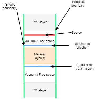
To get a spectrum in NIDN, the transmission and reflection coefficients are calculated by simulating twice for each frequency, one time with the material and one time in vacuum/free space. The transmission coefficient is computed as the mean square (MS) value of the signal from the material simulation divided by the MS of the signal from the free-space simulation.
The boundaries are periodic in both y and z dimension, in order to simulate an infinite plane, i.e. avoid boundary effects. The boundary in the x direction is a perfectly matched layer (PML), which serves to absorb the entire wave and thus prevent artifacts at the edges of the grid.
The permittivity of the material is given for each frequency by the real part of the permittivity function, and the imaginary part of the permittivity is used to get the correct conductivity of the material, which is how FDTD introduces losses in the material. The conductivity is given by: .. math:
{\sigma}({\omega}) = 2*{\pi}*f*{\epsilon}^{''}*{\epsilon_0}
The image shows how the FDTD simulations are set up. The source is placed at the top, with a PML layer just above to absorb all upward signal and avoid reflections. There is some vacumm/free space before the material, and a detector for the reflection just before the material. Then the material follows, and a new detector is placed after the material to measure the transmission. After the material, there is a layer of vacuum before a PML layer at the end to avoid reflection from the back.
The transmission signal can be used as is, but the reflection signal contains both the forward-going signal, and the reflected signal. Thus, the free-space reflection signal (which is just a forward going wave) is substracted from the material reflection signal, to obtain the true reflection signal. This is based on the assumption that the forward-going signal is the same for the free-space simulation and the material simulation.
The FDTD backend code is a modified version of this: https://fdtd.readthedocs.io/en/latest/index.html. Examples of how to use the FDTD simulations can be found in the Running_FDTD.ipynb notebook.
Neural Inverse Design
NIDN is based on a machine learning (ML) approach by Mildenhall et al. called NeRF. Both the NeRF network and similar ones, like sinusoidal representation networks (SIRENs), are available in NIDN.
Our inverse design framework
The difference between our NeRF-based framework and many other types of inverse design is that the we use backpropagation. In our case, the process is based on an iterative trial-and-error approach where the neural network inputs some initial geometry to the simulation and gets feedback on how far from the desired spectrum it was through error backpropagation. The focus is only on the task at hand (solving one solution - a specific spectrum/spectra), while for other inverse design frameworks the neural network must often solve the entire solution space of the problem. The result is that our approach is much more efficient.
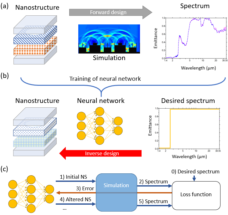
Figure 1: Overview of design processes. (a) Conventional forward design process. (b) Typical inverse design process. Results from (a) are fed into the neural network that subsequently finds the geometry for the desired spectrum. (c) Out NeRF-based inverse design process with backpropagation. The process is based on an iterative trial-and-error approach where the neural network inputs some initial nanostructure (NS) geometry to the simulation and gets feedback on how far from the desired spectrum it was.
Direct epsilon estimation (regression)
One approach NIDN takes to get to the desired property of the material is with direct estimation of the dielectric constant - called direct epsilon estimation or regression. If you want to find, for instance, the dielectric constant for each layer or grid point in a structure such that the reflection, transmission, and absorption (RTA) satisfies your needs, then NIDN can give an estimate of the unrestricted dielectric constant for each frequency.
Utilizing real materials (classification)
The drawback with regression is that the dielectric constant for each frequency is not necessarily resembling that of a real material. To make the problem more realistic, NIDN can also classify which material has a dielectric constant for each frequency closest to the estimated one.
A problem with classification is that the selection of real materials can break the differentiability of the network. Currently, torch doesn’t allow differentiability of the argmax function. As a solution, we {Pablo fill in}.
To be able to classify materials, we must have a library of material properties available. For TRCWA, that means knowing the dielectric constant as a function of frequency of the light. We are in the process of collecting more materials. If you know any good sources of materials over large spectra, feel free to let us know.
Running NIDN
We are now ready to get started. Before we go ahead, we must do the imports.
Imports
### Imports (TODO remove this when finished)
%load_ext autoreload
%autoreload 2

# Append root folder in case you haven't installed NIDN
import sys
sys.path.append("../")

import nidn
Setting the target spectra
The goal of using NIDN is to find a structure with reflection, transmission, and reflection spectra as close to you target spectra as possible. We might for instance want a filter that has a high transmission for wavelengths around 1.4 μm and low transmission for other wavelengths. The reflection should be opposite to that of the transmission and the absorption should be minimal for all wavelengths. The target spectra with these requirements can be set using the following code:
# Load default cfg as starting point
cfg = nidn.load_default_cfg()

# Can we here set the wavelength range?

# Let's investigate 20 frequency points
cfg.N_freq = 20
# Currently, the target spectra is set manually as a list of numbers
cfg.target_reflectance_spectrum =   [1.0]*12 + [0.0]*1 + [1.0]*7 #TODO check that this is correct
cfg.target_transmittance_spectrum = [0.0]*12 + [1.0]*1 + [0.0]*7
# Since R + T + A = 1, we only need to give the reflectance and transmittance (absorptance is implicit)

nidn.plot_spectrum(cfg,
                   cfg.target_reflectance_spectrum,
                   cfg.target_transmittance_spectrum)

physical_wls, normalized_freqs = nidn.get_frequency_points(cfg)
print("Physical wavelengths are (in meters):")
print(physical_wls)
NB: The frequency range is not stable when we change all the time!
What happened in the cell above is that we choose 20 frequency points {logarithmically/linearly} spread between 0.1 and 4 in the frequency domain. In TRCWA, the frequencies are given in relation to the lattice vectors, given in micrometers. A frequency of 0.1 and 4 therefore corresponds to a physical wavelength of (1/0.1) μm = 10 μm and (1/4) μm = 0.25 μm, respectively, as given by nidn.get_frequency_points() function.
If you want to make sure the design target is obtainable, for instance to use it as a ground truth, then you can do a simulation of the spectrum from some structure using the Running_TRCWA notebook.
Examples of how to run NIDN
Now, over to the exciting stuff. In this notebook, we will present three examples. The target spectra in the first and second example have been made using the Running_TRCWA notebook, i.e., they serve as ground truths. The structure used is a uniform single-layer made of titanium oxide. In Example 1, the epsilon is unrestricted, meaning the dielectric constant can take any value within the upper and lower bounds for epsilon for every frequency point. This is what we call regression. In Example 2, we redo Example 1 but using classification, where the material closest to the suggested epsilon is chosen. In Example 3, we find the structure that satisfies the requirements outlined under Setting the target spectra, basically an optical filter.
Example 1 - Uniform single-layer with unrestricted epsilon
Let’s start with a uniform single-layer and see if NIDN can get sufficiently close to the ground truth.
cfg.Nx = 1 # Set layer size  to 1x1 (interpreted as uniform)
cfg.Ny = 1
cfg.N_layers = 5 # Choose number of layers
cfg.type = "regression" # Choose type as described above
cfg.iterations = 2000 # Set number of training iterations (that is forward model evaluations) to perform
#Show all used settings
nidn.print_cfg(cfg)
print_cfg(cfg) shows you more or less everything you want to know
about the config. Using run_training(cfg), we run the network until
it reaches the number of iterations set above (or until you interrupt
it).
nidn.run_training(cfg);
Interpretation of results
Loss plot
The loss as a function of model evaluations is presented below. As the training evolves, the three losses here, L1, Loss, and Weighted Average Loss, can be seen to decrease. {Pablo add link/explanation to the other losses}.
nidn.plot_losses(cfg)
Spectrum plots
The produced RTA spectra are plotted together with the target spectra in the figure below.
nidn.plot_spectra(cfg)
Absolute grid values plot
The complex absolute value of the epsilon over all frequencies is presented here. This plot is in general more useful for patterned multilayers.
nidn.plot_model_grid(cfg)
Epsilon vs frequency and real materials
The following function plots the epsilon values vs. frequency of grid points against real materials in our library. This plot is in general more useful for patterned multilayers.
nidn.plot_eps_per_point(cfg)
Example 2 - Uniform single-layer with materials classification
Next up is the same example, a uniform single-layer of titanium oxide, but this time we check if NIDN can predict the correct material.
cfg.pop("model",None); # Forget the old model
cfg.Nx = 16 # Set layer size  to 16x16 (each of the grid points has its own epsilon now)
cfg.Ny = 16
cfg.eps_oversampling = 4
cfg.N_layers = 2 # Less layer to keep compute managable
cfg.type = "regression" # Choose type as described above (for now still regression)
cfg.iterations = 250 # Set number of training iterations (that is forward model evaluations) to perform
nidn.run_training(cfg);
nidn.plot_losses(cfg)
nidn.plot_spectra(cfg)
nidn.plot_model_grid(cfg)
nidn.plot_eps_per_point(cfg)
As can be seen from the plots, the prediction is correct and, unsurprisingly, the loss is even lower.
Example 3 - Optical filter with regression
For the third and final example, we will try to find the structure that satisfies the requirements outlined under Setting the target spectra using regression. The structure would work as an optical filter with transmission only for wavelengths around 1.4 micrometers. The structure consists of Y layers with X x X grid points per layer. As can be seen in the code below, we make use of oversampling.
cfg.pop("model",None); # Forget the old model
cfg.Nx = 16 # Set layer size  to 16x16 (each of the grid points has its own epsilon now)
cfg.Ny = 16
cfg.eps_oversampling = 8
cfg.N_layers = 2 # Less layer to keep compute managable
cfg.type = "classification" # Choose type as described above (for now still regression)
cfg.iterations = 250 # Set number of training iterations (that is forward model evaluations) to perform
nidn.run_training(cfg);
Interpretation of results
# The other plots
nidn.plot_losses(cfg)
nidn.plot_spectra(cfg)
nidn.plot_model_grid(cfg)
nidn.plot_eps_per_point(cfg)
NIDN is able to get quite close to the desired spectra with the unrestricted epsilon.
Material ID plot
Finally, we will present another plot, showing the real materials closest to the unrestricted ones for each grid point. The layers are numbered from bottom to top, and the light is incident on the first layer, i.e., the bottom of the stack.
nidn.plot_material_grid(cfg)
NB Here we should have plotted the RTA result of this structure.
Saving your plots
In case you want to save results you can use this handy function to save it to the results folder with a current timestamp.
nidn.save_run(cfg)

# You can save all available plots to a single folder using this function
nidn.save_all_plots(cfg,save_path="/results/example/")
Parameters to configure
The following are the parameters in the default_config.toml file, with a short explanation with datatype and the function of the variable
Neural Network parameters
Training Properties
name (str): The name you choose to call the model
use_gpu (bool) : true or false. Whether to use gpu for calculations (true) or cpu (false)
seed (int) : Random seed for the training, in order to be able to reproduce result
model_type (str) : “siren” or “nerf”. What type of model architecture to use
iterations (int) : number of iterations in training the neural network
learning_rate (float) : The learning rate for the training of the neural network, a higher value leads to larger steps along the gradient. Reduce if problems occur.
type (str) : “classification” or “regression”. For more details see notebooks in the repository.
reg_loss_weight (float) : weighting of the regularization loss, only used in classification to force the network to pick one material.
use_regularization_loss (bool) : Only relevant for classification, activates the regularization.
Loss
L (float) : The exponent of the loss, e.g. L=2 leads to a L2 loss, L=1 leads to mean absolute error (L1 loss)
absorption_loss (bool) : Whether to include the absorption spectrum in the loss function.
Model Parameters
n_neurons (int): Number of neurons in the neural network
hidden_layers (int) : Number of hidden layers in the model
encoding_dim (int) : Dimension of the encoding of the model.
siren_omega (float) : Omega value for the siren model, see paper.
Epsilon Properties
add_noise (bool) : Whether to add small noise to output of the network, to avoid getting stuck in local minima.
noise_scale (float) : Scale of the added noise
eps_oversampling (int) : Oversampling of the network output (e.g. network produces 3x3 grid with eps_oversampling = 3, solver uses 9x9)
real_min_eps (float) : The minimum real part of epsilon the model may use
real_max_eps (float) : The maximum real part of epsilon the model may use
imag_min_eps (float) : The maximum imaginary part of epsilon the model may use
imag_max_eps (float) : The maximum imaginary part of epsilon the model may use
avoid_zero_eps (bool) : Whether the epsilon value is allowed to be zero (Would break FDTD to have a epsilon value of 0)
Simulation type
solver (str) : Options are “TRCWA” and “FDTD”
Grid dimensions
Nx (int) : Number of grid-points in x-direction (wave propagating in z-direction). Should only be different than one for patterned layers.
Ny (int) : Number of grid-points in y-direction (wave propagating in z-direction). Should only be different than one for patterned layers.
N_layers (int) : Number of layers of material in simulation
PER_LAYER_THICKNESS (array[float]) : Array of thickness for each material layer. Should be the same length as N_layers, or length one iff all layers are of same size
physical_wavelength_range (tuple[float, float]): Minimum and maximum wavelength to simulate
freq_distribution (str): “linear” or “log”. How the frequencies should be distributed between min and max frequency
N_freq (int) : Number of frequencies to use in the simulation
target_reflectance_spectrum (array[float]) : The reflection spectrum to try to match. Should be of length N_freq
target_transmittance_spectrum (array[float]) : The transmission spectrum to try to match. Should be of length N_freq
TRCWA parameters
TRCWA_L_grid [[float,float],[float,float]]) : physical grid dimension for TRCWA in UNIT_MAGNITUDE (defaults to µm), e.g [[0.1,0.0],[0.0,0.1]]
TRCWA_NG (int) : Truncation order, see TRCWA documentation
FDTD parameters
These are parameters that decides how the FDTD simulation is set up.
FDTD_source_type (str) : The geometry of source, either “point” for pointsource or “line” for linesource. Experiments suggest unexpected reflfctions when using a point source with periodic boundaries.
FDTD_pulse_type (str) : What type of signal is sent out by the source, either a pulse or continuous wave. “hanning”, “ricker” or “continuous” accepted. Hanning is a pulse which windows a continuous wave, while ricker is a pulse with the form ogf the second derivative of a guassian, giving a mean value of zero.
FDTD_pml_thickness (float): Thickness of PML layer in FDTD simulations, set in FDTD unit magnitudes. Perfectly Matched Layer are boundaries used in the x-direction, design to absorb all radiation. (Heard someone say that this should be minimum the largest wavelength)
FDTD_source_position (tuple[float,float]): Coordinates of the source used in FDTD simulations, in FDTD unit magnitudes. Given as a tuple, [x,y]
FDTD_free_space_distance (float): The thickness of the free space layer before and after the material layers, in FDTD unit magnitudes
FDTD_niter (int): Number of timesteps used in FDTD simulation.
FDTD_gridpoints_from_material_to_detector (int) : Distance between material and detectors in grid points. Distance to reflection detector from start of the material, and to from the end of the material to the transmission detector.
FDTD_min_gridpoints_per_unit_magnitude (int) : Minimum number of gridpoints per unit_magnitude, ensuring enough gridpoints for proper functionallity